
Get to know the mathematics behind stock price modelling
According to classical mechanics, the macroscopic world around us evolves in a completely deterministic fashion, where the effect of every cause can, in principle, be computed beforehand. The immense complexity of the real word, however, rarely permits us to do so, and hence we often resort to modelling the surrounding phenomena by random (or stochastic) […]

According to classical mechanics, the macroscopic world around us evolves in a completely deterministic fashion, where the effect of every cause can, in principle, be computed beforehand. The immense complexity of the real word, however, rarely permits us to do so, and hence we often resort to modelling the surrounding phenomena by random (or stochastic) methods.
I took some time to write a short introduction to such stochastic differential equations (SDEs) from a mathematical point of view. The focus is on modelling the evolution of a stock price — a use case widely adopted all around the financial world. We will contrast the stock price, which we view as a stochastic process (Figure 3), with the completely predictable (or deterministic) growth of a bank account balance with an interest rate (Figure 1). The latter is a typical example of an ordinary differential equation (ODE).
Qvik has lead application development projects with a number of companies in the financial sector. These kinds of calculations underlie the financial forecasts based on which the investment strategies are made. In layman’s terms, one is interested in creating investment portfolios, which divide the funds between different stocks and bank accounts in an optimal way.
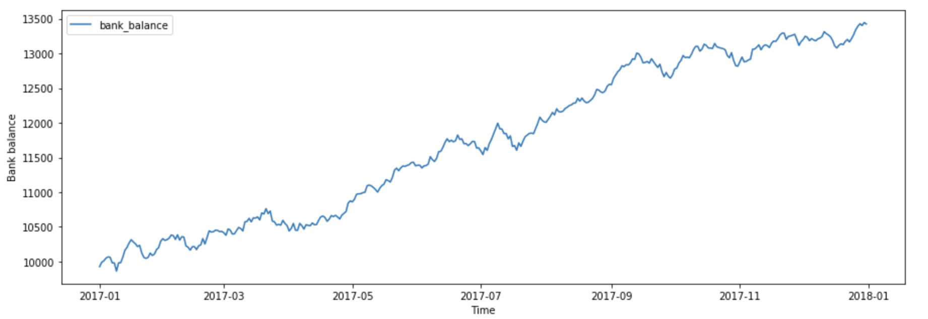
Fig. 1: Growth of a (fictional) bank account balance
Solving the SDE
What are the crucial components of our stock price SDE and how can we solve it so that an understandable plot such as Figure 3 can be produced? The mathematical interpretation of an SDE begins by defining the noise component in a rigorous manner. It turns out that the resulting stochastic process (known as the standard Wiener process) has continuous, but nowhere differentiable, sample paths (Figure 2). Now, solutions to differential equations rely on integration, but integrals with respect to such rough paths lead to surprisingly delicate and thorny issues. This leads us to the theory of stochastic integration.
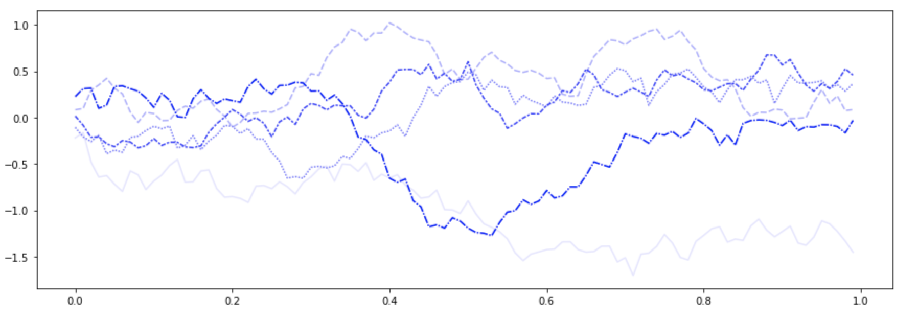
Fig. 2: Sample paths of a standard Wiener process
Our SDE has two parameters, the expected rate of return and volatility both of which we, for simplicity, assume to be constant. In practise their values can be inferred from historical stock data, and in a more realistic scenario we would allow them to vary with time. We will, however, keep our treatment purely mathematical and without any reference to actual stocks. The more detailed discussion can be found in this Jupyter notebook.
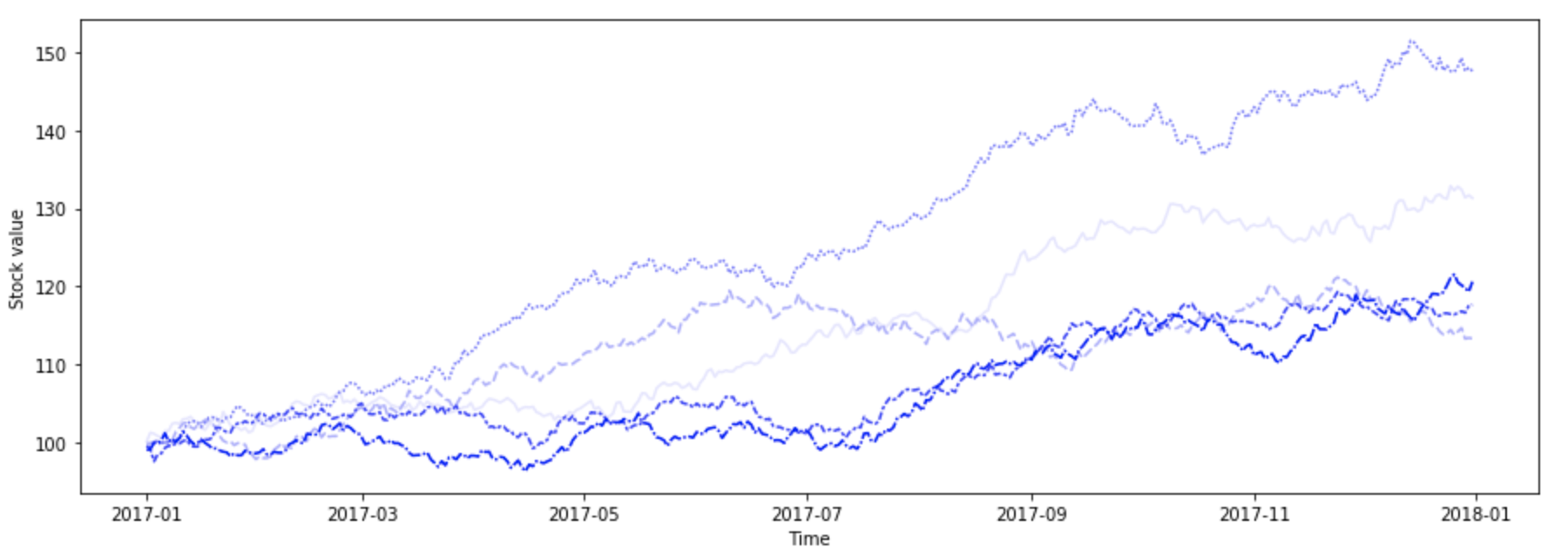
Fig. 3: Possible growth scenarios of a (fictional) stock value
In this blog post we’ve briefly touched the topic of SDEs and their applications in finance. The ability to model stock prices is an great starting point for more advanced problems such as option pricing. I hope this text has sparked interest in the reader to dig deeper and learn more.
For the mathematically minded, the following books will offer plenty of food for thought:
S.Shreve: Stochastic Calculus for Finance I & II
A.N. Shiryaev: Essentials of Stochastic Finance
How does Electrolux create its scalable world-class IoT solutions? By bringing software to the core of the company strategy.

Web push notifications on iPhone and iPad are finally here – but you still need a PWA to use them
How to estimate a budget for your mobile app? We did the maths and can show you.